FlowFields with same filters and table in a single OUTER APPLY

The last blog post about performance improvements in v27 (Dynamics 365 Business Central 2025 Wave 2).

It is a very subtle – but proficient – optimization to what was (and is) called SmartSQL. SmartSQL was introduced – if my mind assists – with NAV 2013 (version 7.0) more than 10 years ago.

(Yeah. Exactly that feature that old navigated on-prem folks used to disable in test environment to measure each single Flow Field T-SQL equivalent statement duration using SQL Profiler.)

Why SmartSQL? Well… This was necessary (a smart move) to reduce the chattiness between SQL and NST nodes. In other words, to reduce the number of SQL Statements sent over network and kill latencies.

With SmartSQL, instead of sending N+1 queries, where N is the number of Flow Fields, only 1 single SQL Statement is sent over with a series of OUTER APPLY in its definition.

Every OUTER APPLY represents, roughly, the data retrieval artifact for one single Flow Field.

Until Now.

With Dynamics 365 Business Central 2025 Wave 2, the platform will automatically pack up into one single OUTER APPLY ALL the Flow Fields that are bound to the same table AND have the same filter.

In a nutshell, all the Flow Fields that perform a different aggregation on the same data pool (SAME Table with SAME Filters) are now part of the SAME OUTER APPLY statement, hence ensuring no duplication in data pool retrieval with a consequent different – faster – execution plan.

Ok. OK… I have explained that. But you probably didn’t get what I mean because it seems like the typical Italian supercazzola (probably you have the same in your country too – it is when someone is playing to be an illusionist, a mentalist, with you -) explained in gestures…

Let’s demonstrate it, then, with a simple scenario, using the demo app that you can find here:

https://github.com/duiliotacconi/DT.AL/tree/main/BC27-Performance-Features

and that defines a super simple customer table like:

// Customer table with FlowFields for demonstration
table 55015 "DT Customer Demo"
{
    Caption = 'Customer Demo';
    DataClassification = CustomerContent;
    fields
    {
        field(1; "Customer No."; Code[20])
        {
            Caption = 'Customer No.';
        }
        field(10; Name; Text[100])
        {
            Caption = 'Name';
        }
        // FlowField demonstrations
        field(101; "No. of Sales Entries"; Integer)
        {
            FieldClass = FlowField;
            Caption = 'No. of Sales Entries';
            CalcFormula = count("DT Sales Entry" where("Customer No." = field("Customer No.")));
            Editable = false;
        }
        field(103; "Last Sales Date"; Date)
        {
            FieldClass = FlowField;
            Caption = 'Last Sales Date';
            CalcFormula = max("DT Sales Entry"."Posting Date" where("Customer No." = field("Customer No.")));
            Editable = false;
        }
    }
    keys
    {
        key(PK; "Customer No.")
        {
            Clustered = true;
        }
    }
}

And Sales Entry is defined as:

// Sales entries table for FlowField calculations
table 55016 "DT Sales Entry"
{
    Caption = 'Sales Entry';
    DataClassification = CustomerContent;
    fields
    {
        field(1; "Entry No."; Integer)
        {
            Caption = 'Entry No.';
            AutoIncrement = true;
        }
        field(10; "Customer No."; Code[20])
        {
            Caption = 'Customer No.';
        }
        field(20; "Posting Date"; Date)
        {
            Caption = 'Posting Date';
        }
        field(30; Amount; Decimal)
        {
            Caption = 'Amount';
        }
        field(40; "Document Type"; Enum "DT Document Type")
        {
            Caption = 'Document Type';
        }
    }
    keys
    {
        key(PK; "Entry No.")
        {
            Clustered = true;
        }
        key(CustomerDate; "Customer No.", "Posting Date")
        {
            SumIndexFields = Amount;
        }
    }
}

Just click on “Flow Field Optimization Demo”, the app will

Create some Customer Demo data
Create some Sales Entry Demo data
Start an AL Profiling session
Run a FindSet with SetAutoCalfields on the Customer Demo Flow Fields
Stop the AL Profiling session
Parse the profile data (instead of download – to make it more easy for you -)
Populate a Temporary Table with the AL Profile Nodes

See below a typical output:

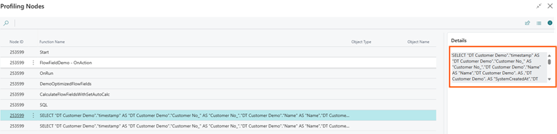
If you copy the SQL Query statement from the “Details” FactBox and format / prettify the output; considering the OUTER APPLYs, you will have something like:

			
SELECT
    "DT Customer Demo"."timestamp" AS "DT Customer Demo"."Customer No_" AS "Customer No_",
    "DT Customer Demo"."Name" AS "Name",
    "DT Customer Demo".AS,
    "DT Customer Demo".AS "SystemCreatedAt",
    "DT Customer Demo".AS "SystemCreatedBy",
    "DT Customer Demo".AS "SystemModifiedAt",
    "DT Customer Demo".AS "SystemModifiedBy",
    ISNULL("SUB$DT Sales Entry$0"."DT Sales Entry$0$No_ of Sales Entries$CNT", 0) AS "No_ of Sales Entries",
    ISNULL("SUB$DT Sales Entry$0"."DT Sales Entry$0$Last Sales Date$MAX$Posting Date", '1753.01.01') AS "Last Sales Date"
FROM
    dbo."CRONUS USA, Inc_$DT Customer Demo" AS "DT Customer Demo" WITH(READCOMMITTED)
    OUTER APPLY (
        SELECT  TOP (1) COUNT("DT Sales Entry$0"."Entry No_")  AS "DT Sales Entry$0$No_ of Sales Entries$CNT",
        MAX("DT Sales Entry$0"."Posting Date") AS "DT Sales Entry$0$Last Sales Date$MAX$Posting Date"
        FROM
            dbo."CRONUS USA, I... )
WHERE (" DT Sales Entry $ 0 "." Customer No_ "=" DT Customer Demo "." Customer No_ ")) AS " SUB $ DT Sales Entry $ 0 " 
ORDER BY " Customer No_ " ASC 
OPTION(OPTIMIZE FOR UNKNOWN, FAST

		

As you might notice, there is just ONE single OUTER APPLY that covers the data needed to calculate “No. of Sales Entries” AND “Last Sales Date”.

In previous versions, you would have noticed TWO OUTER APPLY in the T-SQL query with a consequent different estimated execution plan and redundant data retrieval.

NOTE: if there are maintained indexed views (V-SIFTs) these cannot (and are not, of course) grouped with Flow Fields that are not indexed.

What kind of aggregations can be grouped into one single OUTER APPLY?

SUM / AVERAGE / COUNT
MIN / MAX (NOTE: MIN / MAX could also be grouped with COUNT, if they are indexed)

EXISTS / LOOKUP

CONSIDERATIONS

Microsoft proposes the typical example considering its standard Base Application “G/L Account” where the following filtered WHERE clause:

where(“G/L Account No.” = field(“No.”),

“G/L Account No.” = field(filter(Totaling)),

“Business Unit Code” = field(“Business Unit Filter”),

“Global Dimension 1 Code” = field(“Global Dimension 1 Filter”),

“Global Dimension 2 Code” = field(“Global Dimension 2 Filter”),

“Posting Date” = field(“Date Filter”),

“VAT Reporting Date” = field(“VAT Reporting Date Filter”),

“Dimension Set ID” = field(“Dimension Set ID Filter”)));

It is always the same for “Net Change”, “Debit Amount” and “Credit Amount” Flow Fields.

The same principle is also true for “Budget Credit Amount”, “Budget Debit Amount” that will share one single OUTER APPLY.

… and so on and so forth.

Since this spread all over the application, it might have a good overall impact that could be objectively measured and observed right after upgrading by looking at, for example, pageViews (CL0001) telemetry signals or even traces that contains sqlStatement like e.g. the evergreen Long Running SQL Queries (RT0005).

When you look at it, it seems just a small addition, but it might turn out to give its benefits when you have many Flow Fields that insist on the same table and with the same filter pool.

A good platform feature, then, that is turned always on by default since 27.0.

FlowFields with same filters and table in a single OUTER APPLY

Leave a comment Cancel reply

Subscribe to duiliotacconi.com

Share this:

Related

Leave a comment Cancel reply

Subscribe to duiliotacconi.com